lsodar_bouncing_ball.py

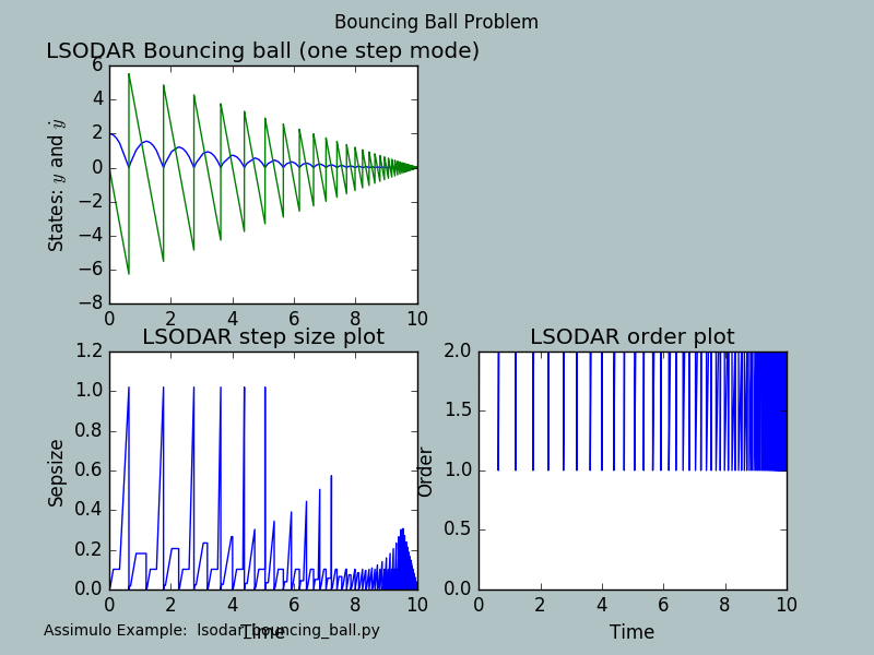
assimulo.examples.lsodar_bouncing_ball.run_example(with_plots=True)

Bouncing ball example to demonstrate LSODAR’s discontinuity handling.

Also a way to use problem.initialize and problem.handle_result in order to provide extra information is demonstrated.

The governing differential equation is

\[\begin{split}\dot y_1 &= y_2\\ \dot y_2 &= -9.81\end{split}\]

and the switching functions are

\[\begin{split}\mathrm{event}_0 &= y_1 \;\;\;\text{ if } \;\;\;\mathrm{sw}_0 = 1\\ \mathrm{event}_1 &= y_2 \;\;\;\text{ if }\;\;\; \mathrm{sw}_1 = 1\end{split}\]

otherwise the events are deactivated by setting the respective value to something different from 0.

The event handling sets

\(y_1 = - 0.88 y_1\) and \(\mathrm{sw}_1 = 1\) if the first event triggers and \(\mathrm{sw}_1 = 0\) if the second event triggers.

---

Warning: Possible chattering detected at t = 9.921283e+00 in state event(s): [0]
Final Run Statistics: Bouncing Ball Problem 

 Number of steps                       : 521
 Number of function evaluations        : 924
 Number of Jacobian evaluations        : 0
 Number of state function evaluations  : 2158
 Number of state events                : 122

Solver options:

 Solver                  : LSODAR 
 Absolute tolerances     : [  1.00000000e-08   1.00000000e-08]
 Relative tolerances     : 1e-06
 Starter                 : classical

Simulation interval    : 0.0 - 10.0 seconds.
Elapsed simulation time: 0.0729551315308 seconds.

Note

Press [source] (to the top right) to view the example.