cvode_with_parameters.py

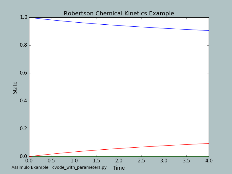
assimulo.examples.cvode_with_parameters.run_example(with_plots=True)

This is the same example from the Sundials package (cvsRoberts_FSA_dns.c) Its purpose is to demonstrate the use of parameters in the differential equation.

This simple example problem for CVode, due to Robertson see http://www.dm.uniba.it/~testset/problems/rober.php, is from chemical kinetics, and consists of the system:

\[\begin{split}\dot y_1 &= -p_1 y_1 + p_2 y_2 y_3 \\ \dot y_2 &= p_1 y_1 - p_2 y_2 y_3 - p_3 y_2^2 \\ \dot y_3 &= p_3 y_ 2^2\end{split}\]

on return:

• exp_mod problem instance
• exp_sim solver instance

---

Final Run Statistics: Robertson Chemical Kinetics Example 

 Number of steps                                       : 147
 Number of function evaluations                        : 168
 Number of Jacobian evaluations                        : 3
 Number of function eval. due to Jacobian eval.        : 9
 Number of error test failures                         : 2
 Number of nonlinear iterations                        : 165
 Number of nonlinear convergence failures              : 0
 Number of sensitivity evaluations                     : 168
 Number of function eval. due to sensitivity eval.     : 1008
 Number of sensitivity nonlinear iterations            : 0
 Number of sensitivity nonlinear convergence failures  : 0
 Number of sensitivity error test failures             : 0

Sensitivity options:

 Method                   : SIMULTANEOUS
 Difference quotient type : CENTERED
 Suppress Sens            : False

Solver options:

 Solver                   : CVode
 Linear multistep method  : BDF
 Nonlinear solver         : Newton
 Linear solver type       : DENSE
 Maximal order            : 5
 Tolerances (absolute)    : [  1.00000000e-08   1.00000000e-14   1.00000000e-06]
 Tolerances (relative)    : 0.0001

Simulation interval    : 0.0 - 4.0 seconds.
Elapsed simulation time: 0.0308549404144 seconds.

Note

Press [source] (to the top right) to view the example.